The riskyData approach
As mentioned in the containers vignette, functions specific to the
data stored the riskyData R6 containers are called methods.
Interaction with them is slightly different to the conventional methods
in R. They can all be applied using the $ operator, meaning
that you don’t have to encapsulate an object within parenthesis.
Available methods
Once you have data imported into R via the loadAPI()
function, the observed data and metadata should sit within an
HydroImport container. Once this is available you can
interrogate the methods available for your data analytics. Interrogation
is very easy, simply apply $methods() to your imported
object.
Again we will use the bewdley example;
data(bewdley)
bewdley$methods()
#> ┌ Methods ───────────────────────────────────────────────────────────────────────────────────┐
#> │ obj$data → Returns the raw data imported via the API │
#> │ obj$rating → Returns the user imported rating details │
#> │ obj$meta() → Returns the metadata associated with the object │
#> │ obj$asVol() → Calculates the volume of water relative to the time step, see ?asVol │
#> │ obj$hydroYearDay() → Calculates the hydrological year and day, see ?hydroYearDay │
#> │ obj$rmVol() → Removes the volume column │
#> │ obj$rmHY() → Removes the hydroYear column │
#> │ obj$rmHYD() → Removes the hydroYearDay column │
#> │ obj$summary() → Provides a quick summary of the raw data │
#> │ obj$coords() → Returns coordinates from the metadata │
#> │ obj$nrfa() → Returns the NRFA data from the metadata │
#> │ obj$dataAgg() → Aggregate data by, hour, day, month calendar year and hydroYear │
#> │ obj$rollingAggs() → Uses user specified aggregation timings, see ?rollingAggs │
#> │ obj$dayStats() → Daily statistics of flow, carried out on hydrological or calendar … │
#> │ obj$quality() → Provides a quick summary table of the data quality flags │
#> │ obj$missing() → Quickly finds the positions of missing data points │
#> │ obj$exceed → Show how many times observed data exceed a given threshold │
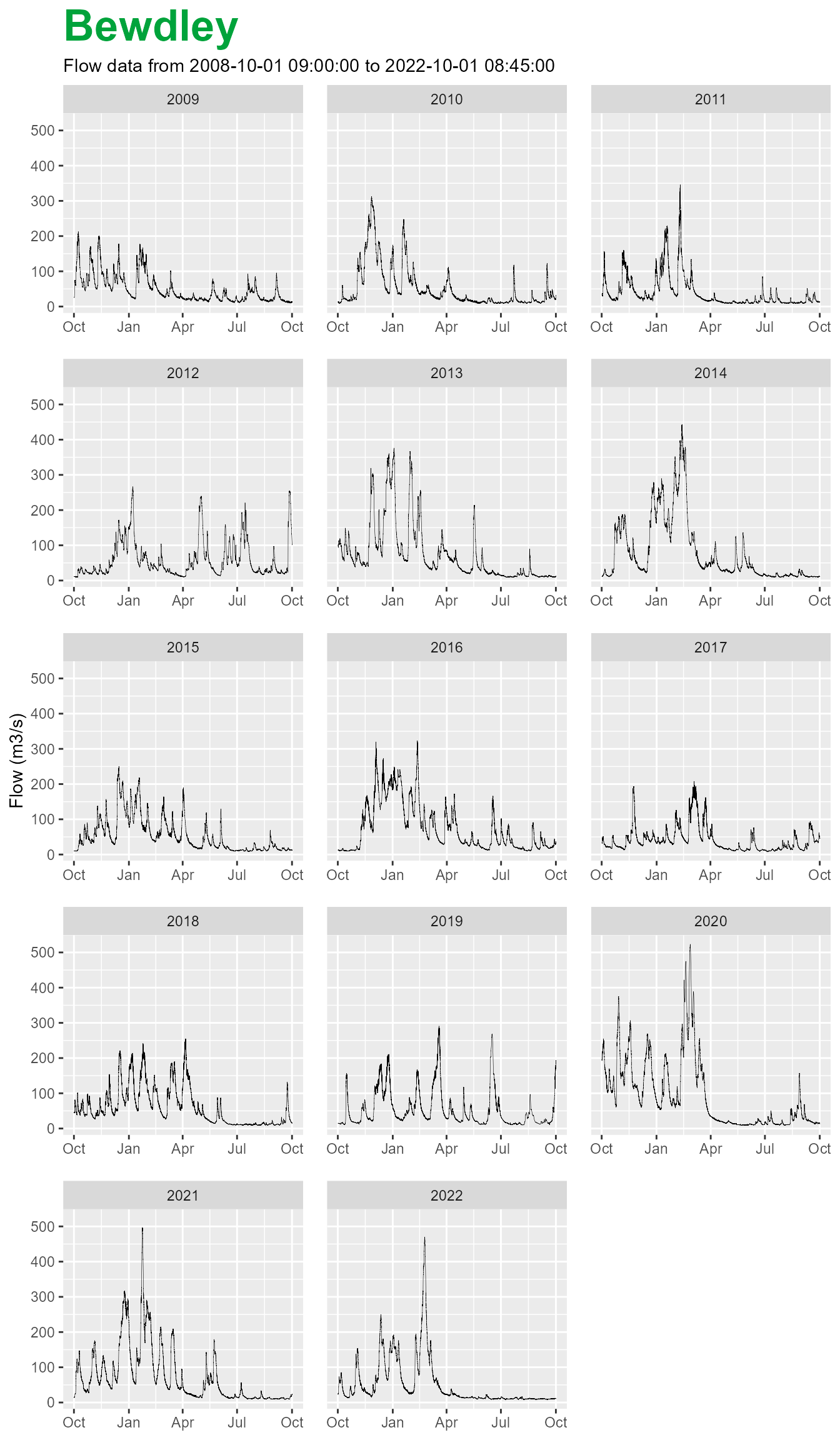
#> │ obj$plot() → Create a plot of each year of data, by hydrological year │
#> │ obj$window() → Extracts the subset of data observed between the times start and end │
#> │ obj$rateFlow() → Converts stage into a rated flow using the specified rating table │
#> │ obj$rateStage() → Converts flow into a rated stage using the specified rating table │
#> └────────────────────────────────────────────────────────────────────────────────────────────┘Accessing data
When the data are imported from the API, they are stored in a public pot within the container. These should be in a data.table format. These provide an enhanced version of data.frame which allows you to do carry out incredibly fast data manipulations. Due to the large size of our data sets it is much more computationally efficient to use over other methods.
To call the data we use $data as you are directly
calling the data and not using a method (or function) we can drop the
parentheses.
bewdley$data
#>                    dateTime value quality  qcode
#>                      <POSc> <num>  <char> <char>
#>      1: 2008-10-01 09:00:00  25.3    Good   <NA>
#>      2: 2008-10-01 09:15:00  25.5    Good   <NA>
#>      3: 2008-10-01 09:30:00  25.6    Good   <NA>
#>      4: 2008-10-01 09:45:00  25.6    Good   <NA>
#>      5: 2008-10-01 10:00:00  25.7    Good   <NA>
#>     ---
#> 490844: 2022-10-01 07:45:00  12.0    Good   <NA>
#> 490845: 2022-10-01 08:00:00  11.8    Good   <NA>
#> 490846: 2022-10-01 08:15:00  11.6    Good   <NA>
#> 490847: 2022-10-01 08:30:00  11.6    Good   <NA>
#> 490848: 2022-10-01 08:45:00  11.6    Good   <NA>
The data available in these can differ between gauge types, the bewdley data in this case is flow. We can see the differences if we look at the chesterton rain gauge dataset;
data(chesterton)
chesterton$data
#>                    dateTime value  valid invalid missing completeness   quality
#>                      <POSc> <num> <char>  <char>  <char>       <char>    <char>
#>      1: 2010-12-31 23:45:00     0      0       0       0   Incomplete Unchecked
#>      2: 2011-01-01 00:00:00     0      0       0       0   Incomplete Unchecked
#>      3: 2011-01-01 00:15:00     0      0       0       0   Incomplete Unchecked
#>      4: 2011-01-01 00:30:00     0      0       0       0   Incomplete Unchecked
#>      5: 2011-01-01 00:45:00     0      0       0       0   Incomplete Unchecked
#>     ---
#> 411969: 2022-10-01 07:45:00     0      0       0     100   Incomplete Unchecked
#> 411970: 2022-10-01 08:00:00     0      0       0     100   Incomplete Unchecked
#> 411971: 2022-10-01 08:15:00     0      0       0     100   Incomplete Unchecked
#> 411972: 2022-10-01 08:30:00     0      0       0     100   Incomplete Unchecked
#> 411973: 2022-10-01 08:45:00     0      0       0     100   Incomplete Unchecked
As you can see the rain gauge data has extra columns. For most analytics the dateTime and value fields are what is used, however it is worth checking if you need to use the extra parameters.
Basic methods
Using the $print() or $summary() methods
can give a quick insight as to what data you have.
bewdley$summary()
#> hydroLoad:
#>  Data Type: Raw Import
#>  Station ID: 2001
#>  Start: 2008-10-01 09:00:00
#>  End: 2022-10-01 08:45:00
#>  Time Zone: GMT
#>  Observations: 490848
#>  Parameter: Flow
#>  Unit Type: m3/s
#>  Unit: http://qudt.org/1.1/vocab/unit#CubicMeterPerSecond
Print works slightly differently, the containers inbuilt print
function overules the one in base R. This means you don’t need to run
$print() you can simply just return the object name.
bewdley
## Works the same as
bewdley$print()
#>
#> ── Class: HydroImport ──────────────────────────────────────────────────────────
#>
#> ── Metadata: ──
#>
#> Data Type: Raw Import
#> Station name: Bewdley
#> WISKI ID: 2001
#> Parameter Type: Flow
#> Modifications: NA
#> Start: 2008-10-01 09:00:00
#> End: 2022-10-01 08:45:00
#> Time Step: 900
#> Observations: 490848
#> Easting: 378235
#> Northing: 276165
#> Longitude: -2.321186
#> Latitude: 52.383072
#>
#> ── Observed data: ──
#>
#>                    dateTime value quality  qcode
#>                      <POSc> <num>  <char> <char>
#>      1: 2008-10-01 09:00:00  25.3    Good   <NA>
#>      2: 2008-10-01 09:15:00  25.5    Good   <NA>
#>      3: 2008-10-01 09:30:00  25.6    Good   <NA>
#>      4: 2008-10-01 09:45:00  25.6    Good   <NA>
#>      5: 2008-10-01 10:00:00  25.7    Good   <NA>
#>     ---
#> 490844: 2022-10-01 07:45:00  12.0    Good   <NA>
#> 490845: 2022-10-01 08:00:00  11.8    Good   <NA>
#> 490846: 2022-10-01 08:15:00  11.6    Good   <NA>
#> 490847: 2022-10-01 08:30:00  11.6    Good   <NA>
#> 490848: 2022-10-01 08:45:00  11.6    Good   <NA>
#> For more details use the $methods() function, the format should be as
#> `Object_name`$methods()
For a quick snapshot on the data quality of the imported data use
$quality()
chesterton$quality()
#>      quality  count
#>       <char>  <int>
#> 1: Unchecked 164581
#> 2:      Good 191351
#> 3:   Missing   2406
#> 4:   Suspect  53635
Accessing the metadata
As mentioned in the container vignette, you can directly interact
with the metadata. This is part of the strict data quality elements that
riskyData enforces. However, should you wish to inspect all
the available metadata for an imported dataset this is simply done with
$meta(). For clarity the table has been transposed by
setting transform = TRUE
bewdley$meta(transform = TRUE)
#>               [,1]
#> dataType      "Raw Import"
#> modifications NA
#> stationName   "Bewdley"
#> riverName     "River Severn"
#> WISKI         "2001"
#> RLOID         "2001"
#> stationGuide  NA
#> baseURL       "http://environment.data.gov.uk/hydrology/id/measures/"
#> dataURL       "8820d897-a09e-4857-8095-5834fee6962f-flow-i-900-m3s-qualified/readings.json?_limit=2000000&mineq-date=2008-10-01&max-date=2022-10-02"
#> measureURL    "8820d897-a09e-4857-8095-5834fee6962f-flow-i-900-m3s-qualified"
#> idNRFA        "54001"
#> urlNRFA       "https://nrfa.ceh.ac.uk/data/station/info/54001.html"
#> easting       "378235"
#> northing      "276165"
#> latitude      "52.38307"
#> longitude     "-2.321186"
#> area          "4325"
#> parameter     "Flow"
#> unitName      "m3/s"
#> unit          "http://qudt.org/1.1/vocab/unit#CubicMeterPerSecond"
#> datum         NA
#> boreholeDepth NA
#> aquifer       NA
#> start         "2008-10-01 09:00:00"
#> end           "2022-10-01 08:45:00"
#> timeStep      "900"
#> timeZone      "GMT"
#> records       "490848"
Other metadata functions include;
## Coordinates of gauges
chesterton$coords()
#>    stationName  WISKI Easting Northing Latitude Longitude
#>         <char> <char>   <int>    <int>    <num>     <num>
#> 1:  Chesterton 164163  512830   294610 52.53766 -0.337867

## NRFA details
bewdley$nrfa()
#>     WISKI codeNRFA                                             urlNRFA
#>    <char>   <char>                                              <char>
#> 1:   2001    54001 https://nrfa.ceh.ac.uk/data/station/info/54001.html
Adding to the public data
Though you could add any number of extra elements to the public data,
the riskyData containers currently have a couple of useful
methods.
If you wished to convert flow into a volume us the
$asVol method;
bewdley$asVol()This adds a volume column to the data table. It uses the metadata to
derive the suitable values based on the difference in time between
observations. If you wished to remove the column use
``$rmVol();
bewdley$rmVol()The other useful method is $hydroYearDay() this
generates 2 things;
Hydrological year (defaults to 1st October to 30 September)
Hydrological day
bewdley$hydroYearDay()
bewdley$data
#>                    dateTime value quality  qcode hydroYear hydroYearDay
#>                      <POSc> <num>  <char> <char>     <num>        <num>
#>      1: 2008-10-01 09:00:00  25.3    Good   <NA>      2009            1
#>      2: 2008-10-01 09:15:00  25.5    Good   <NA>      2009            1
#>      3: 2008-10-01 09:30:00  25.6    Good   <NA>      2009            1
#>      4: 2008-10-01 09:45:00  25.6    Good   <NA>      2009            1
#>      5: 2008-10-01 10:00:00  25.7    Good   <NA>      2009            1
#>     ---
#> 490844: 2022-10-01 07:45:00  12.0    Good   <NA>      2022          365
#> 490845: 2022-10-01 08:00:00  11.8    Good   <NA>      2022          365
#> 490846: 2022-10-01 08:15:00  11.6    Good   <NA>      2022          365
#> 490847: 2022-10-01 08:30:00  11.6    Good   <NA>      2022          365
#> 490848: 2022-10-01 08:45:00  11.6    Good   <NA>      2022          365
Similarly to remove the columns you can remove the hydrological year
with $rmHY() and the hydrological day with
$rmHYD();
bewdley$rmHY()
bewdley$rmHYD()